GWAS (Genome-wise association study) is the one way to find disease-relate-variants.
As a prior to analyze data, QC (quality control) is needed.
I have been using plink for QC and python for manipulating and visualizing data.
If you have vcf files instead of plink formated files, then convert to plink format.
$ plink2 --vcf data.vcf --set-missing-var-ids @_#_\$r_\$a --new-id-max-allele-len 100 --make-bed --out data
or
$ plink2 --vcf data.vcf.gz --set-missing-var-ids @_#_\$r_\$a --new-id-max-allele-len 100 --make-bed --out data
@: chromosome#: position\$r: reference allele\$a: alt allele
After the files are ready, let us follow the regular procedure for GWAS.
Missingness
- Remove missing variants and samples alternately from 0.1 to 0.01.
$ plink2 --bfile raw_data --geno (0.1~0.01) --make-bed --out ft_missing
$ plink2 --bfile ft_missing --mind (0.1~0.01) --make-bed --out ft_missing
Variant distribution
- Check the number of variants at each frequencies.
$ plink2 --bfile ft_pedigree --freq alt1bins=0.01,0.02,0.03,0.04,0.05,0.1,0.2,0.3,0.4,0.5,0.6,0.7,0.8,0.9,1
  : plink2.afreq.alt1.bins
- The ranges are
[0,0.01),[0.01,0.02),...,[0.4,0.5],(0.5,0.6],...,[0.8,0.9),1.
MAF
- Remove low maf variants less than 0.01. The threshold can be calculated by 10/(number of samples).
$ plink2 --bfile ft_missing --maf 0.01 --make-bed --out ft_maf
- Before removing variatns, you can check the minor allele frequency and counts.
$ plink2 --bfile ft_missing --freq   # alt frequency
  : plink2.afreq
$ plink2 --bfile ft_missing --freq counts   # alt counts
  : plink2.acount
HWE
- Remove genotyping error.(p-value < 1e-50)
$ plink2 --bfile ft_maf --hwe 1e-50 keep-fewhet --make-bed --out ft_hwe_gt
- Remove HWE p-value less than 1e-5.
$ plink2 --bfile ft_hwe_gt --hwe 1e-5 keep-fewhet --make-bed --out ft_hwe
$ plink  --bfile ft_hwe_gt --hwe 1e-5 --keep-allele-order --make-bed --out ft_hwe  # plink1.9 the '--hwe' works only in controls. '--hwe-all' works to cases and controls.
keep-fewhet: When significant population stratification is present, this test can be expected to fail in the too-few-hets direction on some normal variants. When using --hwe for quality control, you probably want to keep these variants.
Reference
- Testing for Hardy-Weinberg equilibrium at biallelic genetic markers on the X chromosome.
- The mid p-value in exact tests for Hardy-Weinberg equilibrium.
If you want to see the case or control only,
$ plink2 --bfile ft_hwe_gt --hwe 1e-5 keep-fewhet --keep-if "PHENO1==control" --make-bed --out ft_hwe
-
HWE holds only under the following assumption,
- Random mating.
- No selection or migration.
- No mutation.
- No population stratification.
- Infinite population size.
-
- Source code : https://csg.sph.umich.edu/abecasis/Exact/index.html
- Eighty Years Ago: The Beginnings of Population Genetics, James F. Crow and William F. Dove, Genetics 119:473–476, 1988.
Evidence for departure from HWE has been userd in many applications of discrete P-values in HWE testing.
- Inferring the existence of natural selection :
- Chanllenging the statistical analysis of forensic DNA profile :
- Detecting genotyping errors :
- Gomes, I., A. Collins, C. Lonjou, N. S. Thomas, J. Wilkinson et al., 1999 Hardy-Weinberg quality control. Ann. Hum. Genet. 63: 535–538.
- Zou, G. Y., and A. Donner, 2006 The merits of testing Hardy-Weinberg equilibrium in the analysis of unmatched case-control data: a cautionary note. Ann. Hum. Genet. 70: 921–933.
Relatives
- Remove all first-degree relations.
$ plink2 --bfile ft_hwe --king-cutoff 0.177 --make-bed --out ft_ped
- Duplicate/MZ twin : > 0.354
- First-degree : [0.177, 0.354]
- Second-degree : [0.0884, 0.177]
- Third-degree : [0.0442, 0.0884]
Linkage disequilibrium
: In population genetics, linkage disequilibrium is the non-random association of alleles at different loci in a given population.[WIKIPEDIA]
$ plink2 --bfile ft_ped --indep-pairwise 1500 150 0.7  # window size = 1500 bp
$ plink2 --bfile ft_ped --indep-pairwise 1500kb 1 0.7  # if the window size unit is kb, the step is set to be 1.
$ plink2 --bfile ft_ped --indep 1000 100 2  # window size, step, the VIF(variance inflation factor) threshold: 1/(1-R^2)
  : plink2.prune.in , plink2.prune.out

$ plink2 --bfile ft_ped --extract plink2.prune.in --make-bed --out ft_ld
- Recombination unit is CM(centi-morgan). It is approximately 1 Mb. So LD should be within the size.
- R2 : to remove SNPs if R2 is not less than 0.7.
- plink2.prune.in : R2 >= 0.7
- plink2.prune.out : R2 < 0.7
- VIF = 1 : completely independent
- VIF = 2~10 : usual cut-off
Check the correlation between SNPs.
$ plink --bfile ft_ped --keep-allele-order --r2 dprime with-freqs --ld-window 999999 --ld-window-kb 1.5 --ld-window-r2 0.7 --out ft_ld
-
pruning: it uses the first SNP (in genome order) and computes the correlation with the following ones (e.g. 50). When it finds a large correlation, it removes one SNP from the correlated pair, keeping the one with the largest minor allele frequency (MAF), thus possibly removing the first SNP. Then it goes on with the next SNP (not yet removed). So, in some worst case scenario, this algorithm may in fact remove all SNPs of the genome (expect one).
-
clumping; it uses some statistic (usually p-value in the case of GWAS/PRS) to sort the SNPs by importance (e.g. keeping the most significant ones). It takes the first one (e.g. most significant SNP) and removes SNPs that are too correlated with this one in a window around it. As opposed to pruning, this procedure makes sure that this SNP is never removed, keeping at least one representative SNP by region of the genome. Then it goes on with the next most significant SNP that has not been removed yet. In the case of computing principal components, there is no p-value available, so I propose to use the MAF instead as the statistic to rank SNPs (in decreasing order). Using MAFs makes clumping very similar to pruning, but without any worst-case scenario.
from https://www.biostars.org/p/343818/.
PCA
$ plink2 --bfile ft_ld --pca
  : plink2.eigenvec , plink2.eigenval
Association
- Logistic regression.
$ plink2 --bfile ft_ld --glm allow-no-covars --ci 0.95 --adjust
equivalently,
$ plink --bfile ft_ld --keep-allele-order --logistic --ci 0.95 --adjust
- Chi-square test.
$ plink --bfile ft_ld --keep-allele-order --assoc --ci 0.95 --adjust
-Fisher's test.
$ plink --bfile ft_ld --keep-allele-order --fisher --ci 0.95 --adjust
https://www.cog-genomics.org/plink/2.0/assoc#glm http://zzz.bwh.harvard.edu/plink/anal.shtml
--adjust qq-plot: checks the overall distribution on test statistics. (only works in plink1.x not in plink2. In the plink2 manual,--adjust cols=+qqis the same function, but it does not work.)--pfilter 1e-3: only report statistics with p-values less than 1e-3.-
lambda: median(chi-square)/0.455 for one degrees of freedom. -
If the variant has less than the conservative threshold of p-value (Bonferroni-corrected threshold : 0.05/(number of variants)) in association test, we can say the variant is significant.
Weight
- Give some weight to samples from covariant quantities.
$ plink2 --bfile ft_ld --glm --covar ft_pca.eigenvec --covar-name PC1 --covar-quantile-normalize PC1 --ci 0.95 --adjust
--covar-quantile-normalize: Normalize covariant quantitle to normali distribution, N(0,1).
Sex info
$ plink2 --bfile ft_ld --check-sex
- Male (1) : XHE > 0.80
- Female (2) : XHE < 0.20
- No sex (0) : 0.20 < XHE < 0.80
PRS
$ plink2 --bfile ft_ld --score plink.PHENO1.glm.logistic.hybrid 2 6 10 header sum
or
$ plink --bfile ft_ld --lasso
$ plink --bfile ft_ld --score plink.lasso 2 header sum
- The score file need to have ID(2), A1(risk allele)(6), OR(10).
https://www.cog-genomics.org/plink/1.9/score
Inbreeding : F
$ plink --bfile sample5 -het
  : plink.het
- F=(observed hom. count - expected count) / (total observations - expected count)
https://www.cog-genomics.org/plink/1.9/formats#het
Heterozygosity : |f| = (1-O/E) < 0.1
$ plink --bfile sample5 --hardy
  : plink.hwe
In 'plink.hwe', there are observed and expected frequencies of heterozygosity for each variants.
import pandas as pd

df=pd.read_csv('plink.hwe', sep='\s+')

df['F']=1-df['O(HET)']/df['E(HET)']
df['abs(F)']=abs(df['F'])
df=df[df['abs(F)'] < 0.1]
df_snp=df['SNP']
df_snp.to_csv('hetero_prune.out',index=False)
$ plink --bfile sample5 --extract hetero_prune.out --recode --out hetero_prun
  : hetero_prun.ped + hetero_prun.map
IBD : PI-HAT > 0.2
: It requires at least 1000 independent SNPs.
- Identical twins, and duplicates, are 100%identical by descent (Pihat 1.0)
- First-degree relatives are 50% IBD (Pihat 0.5)
- Second-degree relatives are 25% IBD (Pihat 0.25)
- Third-degree relatives are 12.5% equal IBD (Pihat 0.125)
$ plink --file hetero_prun --genome --genome-full --min 0.2 # --max 0.5
  : plink.genome
import pandas as pd

df=pd.read_csv('plink.genome',sep='\s+')

ys, xs, patches=plt.hist(df['PI_HAT'].values,bins=[0,0.125,0.25,0.5,1],rwidth=0.8)
for i in range(0, len(ys)):
    plt.text(x=xs[i], y=ys[i],
             s=int(ys[i]),#s='{:0>4.1f}%'.format(ys[i]),
             fontsize=8,
             color='red')
y_min, y_max = plt.ylim()
plt.ylim(y_min, y_max+0.05)
plt.yticks([])
plt.xticks([0,0.125,0.25,0.5,1],fontsize=6)
plt.grid(ls='--',alpha=0.6)
plt.show()
Ex) Z(IBD) = (0.4106, 0.0444, 0.5450), PI_HAT = 0.5672, IBS_DIST = 0.943380, IBS = (6, 53, 515)
-
IBS (Identity by State) vs IBD (Identity by Descent)
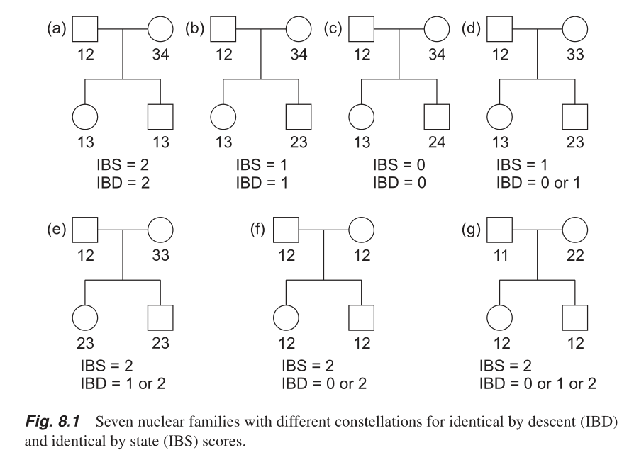
: Chapter 8 in A Statistical Approach to Genetic Epidemiology: With Access to E‐Learning Platform by Friedrich Pahlke, 2nd ed.
-
P(IBD=0)=N(IBS=0)/N(IBS=0|IBD=0)
- P(IBD=1)=[N(IBS=1)-P(IBD=0)N(IBS=1|IBD=0)]/N(IBS=1|IBD=1)
- P(IBD=2)=[N(IBS=2)-P(IBD=1)N(IBS=2|IBD=1)-P(IBD=0)N(IBS=2|IBD=0)]/N(IBS=2|IBD=2)
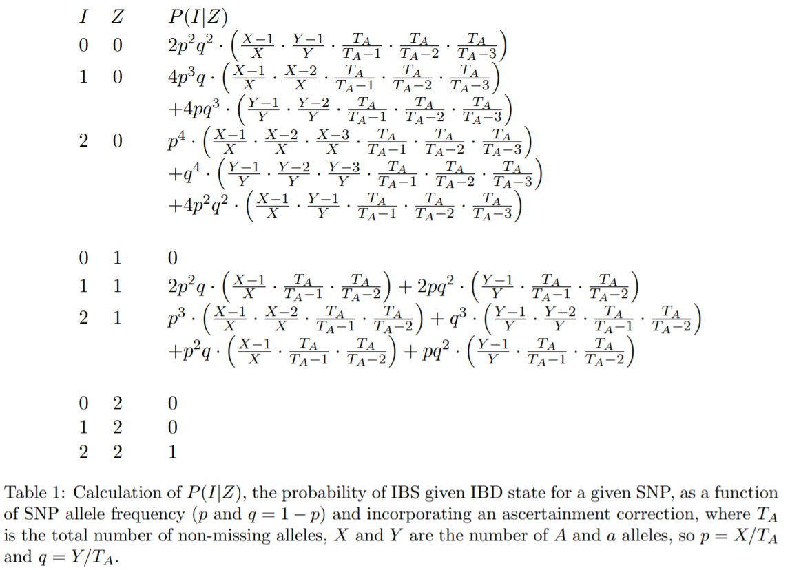
: p12 in PLINK: A Tool Set for Whole-Genome Association and Population-Based Linkage Analyses.
- The IBS method works best when only independent SNPs are included in the analysis.
- Independent SNP set for IBS calcuation is generally prepared by removing regions of extended LD and pruning the remaining regions so that no pair of SNPs within a given window (say, 50kb) is correlated.
- Related individuals will share more alleles IBS than expected by chance, with the degree of additional sharing proportional to the degree of relatedness. http://www.bioinf.wits.ac.za/courses/gwas/OLD/Qc_combined_final.pdf P.18
After imputation
Linear regression : R2 > 0.7
- The linear model regressing each imputed SNP on regional typed SNPs.
MAF > 0.01
Bonferonni-correction : p < 5E-8
Q-Q plot
- To compare observed and expected quantities
LD Block
Low quality SNP
- Genotype clusters of many SNPs demonstrate low quality genotyping due to:
- Low DNA concentration
- Poor binding and competitive binding by other sequences
- Structural and copy number variants
Reference
- A guide to genome-wide association analysis and post-analytic interrogation, https://dx.doi.org/10.1002/sim.6605
- GWAS QC-theory and steps, http://www.bioinf.wits.ac.za/courses/gwas/OLD/Qc_combined_final.pdf